Parallelising a Compile-Time Ray Tracer

Introduction

This is part 3 of the CTRT series. You can read the complete series here:

Last time, we discussed a series of optimisations for the compile-time ray tracer we designed in part 1 along with a way of implementing BRDFs and shadows. In today’s travel, we will continue developing the ray tracer by adding specular shading and reflections. We will also use this as an excuse to discuss how to parallelise the ray tracer. With this in mind, let’s get started by adding specular shading.

Note
At the top of each section, you will find links to all the files that are discussed there in case you want to read the code along with the explanations. The entire source code for this post can be seen here

Ooh… Shiny

The ultimate goal in terms of shading is to have perfect mirror reflections. To do that, we first need to implement specular shading, which we will handle by implementing the Phong specular model. We begin by creating a new BRDF which will be in charge of the specular highlights. The general equation for describing them is as follows:

$$ k_s \cdot c_s \cdot (\mathbf{r} \cdot \mathbf{\omega_o})^{e} $$

Where $k_s$ is the specular reflection coefficient, $c_s$ is the specular colour, $\mathbf{r}$ is the direction of the reflected light, $\mathbf{\omega_o}$ is the viewing direction, and $e$ is the specular exponent. Under normal circumstances, this formula would be implemented like this:

1
specular_reflection * specular_colour * std::pow(r_dot_wo, specular_exponent);

The problem here is that we need std::pow, which is part of the maths functions of the STL… and therefore not constexpr. Since we’re mostly dealing with integral exponents, we can write a simplified version of the pow function as follows:

 1
 2
 3
 4
 5
 6
 7
 8
 9
10
    constexpr float pow(float base, int exp)
    {
        float ret{1.0f};
        for (int i{0}; i < exp; ++i)
        {
            ret *= base;
        }

        return base;
    }

Notice that we’re not going to make it recursive since due to the optimisations we previously discussed (particularly simplifying the call-stack). Now that we have our pow function, we can implement the BRDF as follows:

 1
 2
 3
 4
 5
 6
 7
 8
 9
10
11
12
13
14
15
16
17
18
19
20
21
22
23
24
class GlossySpecular : public BRDF<GlossySpecular>
{
public:
    constexpr GlossySpecular()
    {}

    constexpr Colour
    fn(ShadeRec const& rec, Vector const& wo, Vector const& wi) const
    {
        Colour L;
        float n_dot_wi = dot(rec.normal, wi);
        Vector r{-wi + 2.0f * rec.normal * n_dot_wi};
        float r_dot_wo = dot(r, wo);

        if (r_dot_wo > 0.0f)
        {
            L = m_specular_reflection * m_specular_colour *
                utils::pow(r_dot_wo, m_specular_exponent);
        }

        return L;
    }
    // ...
};

The Phong material is conformed by two BRDFs: the Lambertian BRDF which will handle diffuse shading and the specular BRDF we just wrote. Since we still need to handle shadows, they’re also going to be included in the implementation, and so we end up with this:

 1
 2
 3
 4
 5
 6
 7
 8
 9
10
11
12
13
14
15
16
17
18
19
20
21
22
23
24
25
26
27
28
29
30
31
32
33
34
35
36
37
38
39
40
41
42
43
44
45
46
47
48
49
50
51
52
53
54
55
56
57
58
59
class Phong : public Material<Phong>
{
public:
    constexpr Phong()
    {}

    template<class LightContainer,
             class ShapeContainer>
    constexpr Colour shade(ShadeRec const& rec,
                           LightContainer const& lights,
                           ShapeContainer const& shapes) const
    {
        Vector wo = -rec.ray.direction;
        Colour L  = m_ambient_brdf.rho(rec, wo) * lights[0].l(rec);

        if (lights.size() == 1)
        {
            return L;
        }

        for (std::size_t i{1}; i < lights.size(); ++i)
        {
            Vector wi      = lights[i].get_direction(rec);
            float n_dot_wi = dot(rec.normal, wi);

            if (n_dot_wi > 0.0f)
            {
                bool in_shadow{false};
                if (lights[i].casts_shadows())
                {
                    Ray shadow_ray{rec.hit_point, wi};
                    float d =
                        distance(shadow_ray.origin, lights[i].get_position());
                    for (auto const& shape : shapes)
                    {
                        if (auto result = shape.shadow_hit(shadow_ray); result)
                        {
                            if (*result < d)
                            {
                                in_shadow = true;
                                break;
                            }
                        }
                    }
                }

                if (!in_shadow)
                {
                    L += (m_diffuse_brdf.fn(rec, wo, wi) +
                          m_specular_brdf.fn(rec, wo, wi)) *
                         lights[i].l(rec) * n_dot_wi;
                }
            }
        }

        return L;
    }
    // ...
};

Perfect! Let’s setup a new scene and try it out. After 15 minutes, we end up with the following:

Specular highlights

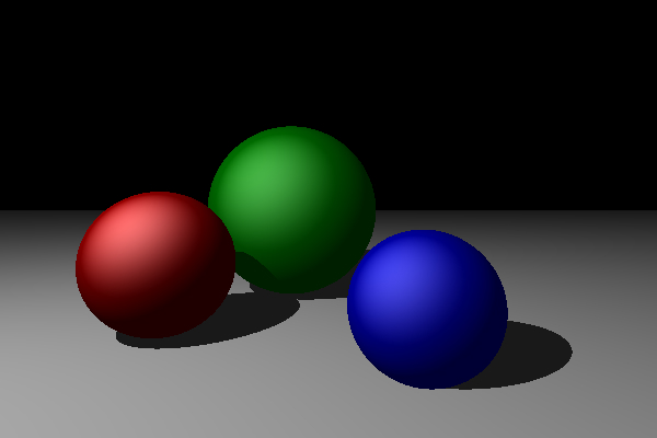
Now that we have specular highlights, lets implement reflections.

Mirror, Mirror, on the Wall…

Since we’re adding a new material, we first have to add a new BRDF. A perfect reflection BRDF is a bit different from the others we’ve written so far, mainly because we are not interested in evaluating the BRDF function. Indeed, in a perfect mirror, the colour of the surface is not determined by the surface, but rather by the colour of the surfaces that are reflected on it and the base colour of the reflective surface itself. To fully understand this, imagine a perfect mirror. The colours on the mirror are entirely dependent on whatever is being reflected on it. Now suppose we tint the mirror with a colour (say red). The resulting colour on the surface of the mirror is composed of the red tint and whatever is being reflected.

What we’re actually interested in is not the evaluation of the BRDF itself, but rather the direction in which the rays are going to be reflected and the base colour of the mirror (if any). Therefore, we’re going to be adding a new function to our BRDF base class:

 1
 2
 3
 4
 5
 6
 7
 8
 9
10
11
template<typename T>
class BRDF : public utils::StaticBase<T, BRDF>
{
public:
    // ...
    constexpr std::tuple<Colour, Vector> sample_fn(ShadeRec const& sr,
                                                   Vector const& wo) const
    {
        return this->self().sample_fn(sr, wo);
    }
};

Notice that due to the usage of CRTP, every time we add a function to the base class, we must implement it in all the derived classes (otherwise the compiler will issue a warning/error about infinite recursion on the base class since it ultimately calls itself). For all of our existing BRDFs, sample_fn will return a default tuple. Now that this is done, we can create a new BRDF:

 1
 2
 3
 4
 5
 6
 7
 8
 9
10
11
12
13
14
15
class PerfectSpecular : public BRDF<PerfectSpecular>
{
public:
    constexpr std::tuple<Colour, Vector> sample_fn(ShadeRec const& sr,
                                                   Vector const& wo) const
    {
        float n_dot_wo = dot(sr.normal, wo);
        Vector out_vec = -wo + 2.0f * sr.normal * n_dot_wo;
        Colour out_col =
            m_reflection_coeff * m_reflection_colour / dot(sr.normal, out_vec);

        return {out_col, out_vec};
    }
    // ...
};

The naming is due to the fact that the previous BRDF that we created is used to create glossy specular (so not perfect) reflection, whereas this one will generate pure specular reflections. Now that this is set, we need to discuss the material itself.

In general, reflections in ray tracing are handled through recursive function calls. A very simple version of this would involve something like this:

1
2
3
4
5
6
Colour reflective_shade(ShadeRec const& sr, World const& w)
{
    <Compute base shade>;
    <Compute reflected ray>;
    w.trace(ray);
}

This is fine if we aren’t dealing with the restrictions of constexpr. Since we are, then we have to be a bit more careful. The recursive call still has to happen, but the question now is where. Looking through our current setup, it turns out that it is a lot easier to have the materials themselves be recursive, since those are the only ones that deal with the colour computations. So, we would be changing the shade function as follows:

 1
 2
 3
 4
 5
 6
 7
 8
 9
10
11
12
    constexpr Colour shade(ShadeRec const& sr,
                           LightContainer const& lights,
                           ShapeContainer const& shapes,
                           MaterialContainer const& materials) const
    {
        <Compute base shade>;
        <Compute reflected ray>;

        <for each shape in scene>:
            <if reflected ray hits shape>:
                <add colour contribution>;
    }

In order to do this, we’re going to need to pass the container of shapes down to the shade function. This is simple enough, all we have to do is tack on another template parameter to the base shade class and propagate the changes. The new base shade function ends up looking like this:

 1
 2
 3
 4
 5
 6
 7
 8
 9
10
11
12
13
14
15
template<typename T>
class Material : public utils::StaticBase<T, Material>
{
public:
    template<class LightContainer,
             class ShapeContainer,
             class MaterialContainer>
    constexpr Colour shade(ShadeRec const& rec,
                           LightContainer const& lights,
                           ShapeContainer const& shapes,
                           MaterialContainer const& materials) const
    {
        return this->self().shade(rec, lights, shapes, materials);
    }
};

Now that we have the base ready to go, let’s create the new reflective material:

 1
 2
 3
 4
 5
 6
 7
 8
 9
10
11
12
13
14
15
16
17
18
19
20
21
22
23
24
25
26
27
28
29
30
31
32
33
34
35
36
37
38
39
40
41
42
class Reflective : public Material<Reflective>
{
public:
    template<class LightContainer,
             class ShapeContainer,
             class MaterialContainer>
    constexpr Colour shade(ShadeRec const& sr,
                           LightContainer const& lights,
                           ShapeContainer const& shapes,
                           MaterialContainer const& materials) const
    {
        if (sr.reflection_depth > ShadeRec::max_reflection_depth)
        {
            return Colour{0.0f};
        }

        // Direct illumination first.
        Colour L = m_phong.shade(sr, lights, shapes, materials);

        Vector wo     = -sr.ray.direction;
        auto [fr, wi] = m_reflective_brdf.sample_fn(sr, wo);
        Ray reflected_ray{sr.hit_point, wi};

        Colour reflected_colour;
        for (auto const& shape : shapes)
        {
            if (auto result = shape.hit(reflected_ray); result)
            {
                auto rec             = *result;
                rec.reflection_depth = sr.reflection_depth + 1;
                reflected_colour     = materials[rec.material_id].shade(
                    rec, lights, shapes, materials);
                break;
            }
        }

        L += fr * reflected_colour * dot(sr.normal, wi);

        return L;
    }
    // ...
};

There’s a couple of things to unpack here, so let’s go one at a time. Since reflections are recursive process, we need a base case in order to not have infinite recursion. To handle this, we’re going to add two now elements to the ShadeRec structure: a counter and a maximum reflection depth. Since the counter is always initialised to 0, we just have to make sure we copy (and increase) the current counter whenever we pass it down to the next material to shade. The base case is handled first: if we have exceeded the reflection limit, just return black.

The next bit is the recursion part of the function. Note that we have essentially copied over the code from the main render function. This is on purpose since the code is essentially the same, the only major difference is that we are accumulating the colour from the reflected materials in L. Finally, the “base” colour of the mirror is computed using Phong (this is why we needed to implement it first) so that we can still have specular reflections on it.

We now have a reflective material, so lets test it out. We can take the previous scene and replace a couple of spheres with reflective materials to get this:

Reflections

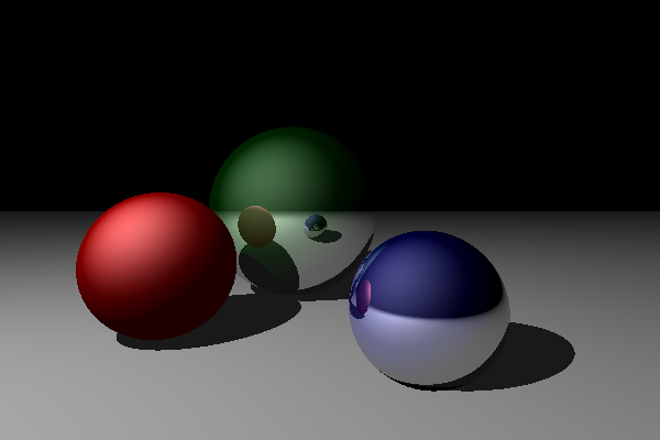
Not bad! Our ray tracer is now pretty capable, but it would be nice if we could somehow make it faster.

How do we Parallelise the Compiler?

Before we begin our discussion, let’s first take note of our current render times:

Scene	Time
Just Background	21m 6s
Red Sphere	11m 43s
Shadows	42m
Phong	15m 33s
Reflections	17m 31s

We have previously discussed several optimisations we could make in our code to increase the performance of the renderer. These improvements led to the times we noted above, but there must be more that we can do. So the question is what?

Let’s forget about the fact that we’re dealing with constexpr functions for a moment and let’s think about what we could do if this were a normal ray tracer. Looking through the algorithm, we can quickly realise that it is trivially parallelisable. In other words, the result of one pixel has no effect on the result of any other pixel in the image. So it would be a simple matter of dividing the pixels among a set number of threads. The best part of this is that because each pixel is entirely independent, we can manage the entire system without any thread locks. This is due to the fact that the scene is read-only (marked const) and the threads will never write to the same pixel, so we don’t need to guard the image itself.

So the new question is this: how do we divide the work among the threads? Well, there are several options we could try:

We could assign a single pixel per thread. This would require some way of dispatching new pixels to the threads once they finish their work (essentially a work queue). This approach is simple but inefficient. The reason is the fact that each pixel won’t take the same amount of time. Therefore it is perfectly possible for threads to finish faster and therefore end up with nothing to do while other threads are locked up in the more complicated pixels. The overall goal of parallelising an algorithm is to ensure that CPU utilisation remains high, so let’s look at other options.
We could divide the image into rows and have each thread do a given row. This is similar to the previous point, but with a larger unit of work. This approach would work well if we had a high number of cores (like the GPU), but this approach is still too similar to the previous one. It is going in the right direction though: since the CPU has a limited number of threads that (in general) will be smaller than the number of rows (or pixels), we need to divide the amount of work into larger chunks.
We could divide the image into regions and assign each region to a thread. These regions (which we will call tiles) would help balance out the work in the threads, since it is easier to have regions that have a mix of both low and high work pixels. Note that it is still possible that we end up with tiles that are mostly empty, but we can reduce that by being a bit clever with the size and distribution of the tiles.

Option number 3 is the most common approach for parallelising ray tracers, so lets go with that. At runtime, we would end up with something like this:

1
2
3
4
5
6
7
render:
    <Divide image into tiles>;
    <Allocate threads>;
    <Assign each tile to a thread>;
    <Launch thread>;
    <Wait>;
    <Write image>;

For the sake of simplicity, lets assume that the number of tiles is equal to the number of threads. The thread render function would have our render function, with the only difference being that instead of an image, it would take the tile, which will tell it where to start and end on each of the two axes.

So, we have an idea of how we would solve it if we weren’t dealing with constexpr functions, so now let’s figure out if we can somehow transfer this over.

If we were to look at the CPU utilisation while we’re running our ray tracer, we would quickly realise that only a single core was being used. Looking through the compiler flags, we are always using the parallel flag, so why isn’t the compiler using multiple threads? Well the answer is simple: we are only ever generating a single executable, so the compiler only needs one thread to generate it… wait. We are generating a single executable, so we are using a single core, so it stands to reason that if we generated multiple executables, we would use multiple cores. But we don’t want multiple executables, so how do we do this… libraries!

Preparing the Tracer

The approach is the same as before: take the image and split it into tiles. The difference is that instead of assigning each thread a single tile, we’re going to be creating a static library per tile. Each library will be in charge of a specific region of the image, which it will then place into an array. All that the main executable needs to do is to loop through all the libraries and retrieve their tiles so they can be assembled into the final image. Perfect! But how do we generate the libraries?

Before we discuss how to generate the libraries themselves, lets modify the core ray tracer to handle tiles instead of the full image. This involves a couple of quick additions and changes. First, we need a tile structure, which will be similar to the Image class. We end up with this:

 1
 2
 3
 4
 5
 6
 7
 8
 9
10
11
12
13
14
15
16
17
18
19
20
21
22
23
24
25
26
27
28
29
30
31
32
33
34
35
36
37
38
39
40
41
42
43
template<class Container,
         std::size_t t_width,
         std::size_t t_height,
         std::size_t image_width,
         std::size_t image_height,
         ImageType type>
class TiledImage
{
public:
    static constexpr std::size_t width{image_width};
    static constexpr std::size_t height{image_height};
    static constexpr std::size_t size{width * height};
    static constexpr std::size_t tile_width{t_width};
    static constexpr std::size_t tile_height{t_height};
    static constexpr std::size_t tile_size{tile_width * tile_height};
    static constexpr int channels{3};

    constexpr TiledImage()
    {
        if constexpr (type == ImageType::dynamic_image)
        {
            m_data.resize(tile_width * tile_height);
        }
    }

    constexpr auto& operator()(std::size_t row, std::size_t col)
    {
        return m_data[(row * tile_width) + col];
    }

    constexpr auto operator()(std::size_t row, std::size_t col) const
    {
        return m_data[(row * tile_width) + col];
    }

    constexpr Container get_data() const
    {
        return m_data;
    }

private:
    Container m_data;
};

Notice that the class is functionally identical to the Image class, the only major difference is that it takes in the size of the image and the tile. The size of the image is important since it used to create the primary rays, while the tile size is used to create and index into the container that holds the pixel data.

Next, let’s modify the render function to accept the tile. The range of the tile will be held by a simple struct:

1
2
3
4
5
6
struct Tile
{
    std::size_t x_start{0}, x_end{0};
    std::size_t y_start{0}, y_end{0};
    std::size_t width{0}, height{0};
};

The new render function looks like this:

 1
 2
 3
 4
 5
 6
 7
 8
 9
10
11
12
13
14
15
16
17
18
19
    template<class Image, class Scene>
    static constexpr void
    render(Image& image, Scene const& scene, Tile const& tile)
    {
        Ray ray;
        ray.origin = scene.get_camera().get_eye();

        const float width  = static_cast<float>(Image::width);
        const float height = static_cast<float>(Image::height);

        auto const& lights    = scene.get_lights();
        auto const& materials = scene.get_materials();
        auto const& shapes    = scene.get_shapes();

        for (std::size_t r{0}; r < tile.height; ++r)
        {
            for (std::size_t c{0}; c < tile.width; ++c)
            {
            // ...

The rest of the function remains the same, as the only changes that were needed happened before the inner loop. Note the declaration of width and height (this is why we needed the image dimensions) and the changes in the two loops to use the size of the tile.

Now that we have everything ready to go, lets turn our attention to the CMake scripts we’ve been using.

Magic with CMake

So far, we’ve been using a single executable, so we could just pass in all of the files into it so they could be compiled. In order to create the new tile libraries, we’re going to have to split our code into 3 blocks:

The core ray tracer: contains the bulk of the code, consisting of the shapes, BRDFs, materials, etc.
The tile libraries: will contain the generator functions for each scene.
The main executable: will be in charge of gathering all the tiles and merging into a single image. Note that this will have to be done at runtime.

With this in mind, our first order of business is to separate the core ray tracing code into a separate library that will be called tracer. For the sake of organisation, we’re going to be placing the files into their own folder (src/tracer). After tweaking the CMake scripts a bit, we are now ready to figure out how to generate the tile libraries.

CMake has a command called configre_file which takes in a template (generally with a .in file extension) and creates a new file. The part that we’re interested in here is that the template can contain special strings that will be replaced when the new file gets created provided that the variable is defined in the CMake script (or any scripts above it). So, we’re going to consolidate all of the common code across the libraries into a single master template that they will all ultimately be copied from. The template will have the strings containing the per-library information that will be substituted when they are created.

Since each library needs to define a single function to retrieve the tile, lets start with the header:

1
2
3
4
5
6
7
8
#pragma once

#include <vector>
#include <tuple>
#include <tracer/vector.hpp>
#include <tracer/renderer.hpp>

std::tuple<std::vector<Colour>, Tile> get_@TILE_NAME@();

When CMake reads this file, it will replace any string (or substring) that begins and ends with @ with the corresponding value in the CMake script itself. So, for the first tile, the get function would become get_tile_0. The cpp template will look like this:

 1
 2
 3
 4
 5
 6
 7
 8
 9
10
11
12
13
14
15
16
17
18
19
20
21
22
23
24
25
26
27
28
29
30
31
32
33
34
35
36
37
38
39
40
41
42
43
#include "@TILE_NAME@.hpp"

#include <tracer/image.hpp>
#include <tracer/scene.hpp>
#include <zeus/timer.hpp>
#include <fmt/printf.h>

constexpr std::size_t image_width{@IMAGE_WIDTH@};
constexpr std::size_t image_height{@IMAGE_HEIGHT@};
constexpr std::size_t tile_width{@TILE_WIDTH@};
constexpr std::size_t tile_height{@TILE_HEIGHT@};

constexpr Tile tile{@TILE_X_START@, @TILE_X_END@, @TILE_Y_START@, @TILE_Y_END@, @TILE_WIDTH@, @TILE_HEIGHT@};

// Generator functions go here...
#if defined(CTRT_RENDER_SCENE_1)
inline auto render_@TILE_NAME@_scene_1()
{
// ...

std::tuple<std::vector<Colour>, Tile> get_@TILE_NAME@()
{
    fmt::print("\nStarting render...\n");
    zeus::Timer<double> timer;
    timer.start();
#if defined(CTRT_RENDER_SCENE_1)
    auto image = render_@TILE_NAME@_scene_1();
#elif defined(CTRT_RENDER_SCENE_2)
    auto image = render_@TILE_NAME@_scene_2();
#elif defined(CTRT_RENDER_SCENE_3)
    auto image = render_@TILE_NAME@_scene_3();
#elif defined(CTRT_RENDER_SCENE_4)
    auto image = render_@TILE_NAME@_scene_4();
#elif defined(CTRT_RENDER_SCENE_5)
    auto image = render_@TILE_NAME@_scene_5();
#endif
    fmt::print("Render finished in: {:.2f}ms\n", timer.elapsed());

    auto image_data = image.get_data();
    std::vector<Colour> data(image_data.begin(), image_data.end());

    return {data, tile};
}

Reading through this code, it may seem odd that we’re using the name of the tile as part of the function signature for the generators. After all, these functions are all defined within the cpp file and therefore aren’t visible outside of the current translation unit… right? Well, it turns out that if we were to compile and run our code without the tile name in the generator functions, we would always be invoking the generator function from the first tile! The reason why this happens is very simple: the functions all have the same names, so when the program gets linked, the linker only accepts the first version of the function (in this case the one corresponding to the first tile) and ignores the rest. In order to prevent this from happening, we need to have each function have a unique name, hence why we use the name of the tile.

We are now ready to modify the script to generate the libraries. The new script looks like this:

 1
 2
 3
 4
 5
 6
 7
 8
 9
10
11
12
13
14
15
16
17
18
19
20
21
22
23
24
25
26
27
28
29
30
31
32
33
34
35
36
37
38
39
40
41
42
43
44
45
46
47
48
49
50
51
52
53
54
55
# Slab information
set(NUM_TILES_HORIZONTAL 1)
set(NUM_TILES_VERTICAL 1)

math(EXPR TILE_WIDTH "${IMAGE_WIDTH} / ${NUM_TILES_HORIZONTAL}")
math(EXPR TILE_HEIGHT "${IMAGE_HEIGHT} / ${NUM_TILES_VERTICAL}")
math(EXPR LOOP_X_END "${NUM_TILES_HORIZONTAL} - 1")
math(EXPR LOOP_Y_END "${NUM_TILES_VERTICAL} - 1")

set(CTRT_TILE_ROOT ${CTRT_SOURCE_ROOT}/tiles)
set(TILE_INPUT_HEADER ${CTRT_TILE_ROOT}/tile.hpp.in)
set(TILE_INPUT_SOURCE ${CTRT_TILE_ROOT}/tile.cpp.in)

set(TILE_TARGET_LIST)
foreach(X RANGE 0 ${LOOP_X_END})
    foreach(Y RANGE 0 ${LOOP_Y_END})
        math(EXPR TILE_X_START "${X} * ${TILE_WIDTH}")
        math(EXPR TILE_Y_START "${Y} * ${TILE_HEIGHT}")
        math(EXPR TILE_X_END "${TILE_X_START} + ${TILE_WIDTH}")
        math(EXPR TILE_Y_END "${TILE_Y_START} + ${TILE_HEIGHT}")

        set(TILE_NAME tile_${X}_${Y})

        # Set the files for the library.
        set(TILE_INCLUDE ${CTRT_TILE_ROOT}/${TILE_NAME}.hpp)
        set(TILE_SOURCE ${CTRT_TILE_ROOT}/${TILE_NAME}.cpp)

        source_group("include" FILES ${TILE_INCLUDE})
        source_group("source" FILES ${TILE_SOURCE})

        # Now generate the files.
        configure_file(${TILE_INPUT_HEADER} ${TILE_INCLUDE})
        configure_file(${TILE_INPUT_SOURCE} ${TILE_SOURCE})

        # Set the library.
        add_library(${TILE_NAME} ${TILE_INCLUDE} ${TILE_SOURCE})
        target_include_directories(${TILE_NAME} PUBLIC ${CTRT_TILE_ROOT})
        target_link_libraries(${TILE_NAME} PUBLIC ctrt_tracer)
        target_compile_features(${TILE_NAME} PUBLIC cxx_std_17)
        target_compile_options(${TILE_NAME} PUBLIC ${CTRT_COMPILER_FLAGS})
        target_compile_options(${TILE_NAME} PUBLIC ${CTRT_DEBUG_FLAGS})
        target_compile_definitions(${TILE_NAME} PUBLIC ${CTRT_COMPILE_DEFINITIONS})
        set_target_properties(${TILE_NAME} PROPERTIES FOLDER "ctrt_tiles")

        if (MSVC)
            set_target_properties(${TILE_NAME} PROPERTIES LINK_FLAGS
                ${CTRT_LINKER_FLAGS})
        endif()

        # Append the new target to the list.
        list(APPEND TILE_TARGET_LIST ${TILE_NAME})
    endforeach()
endforeach()

set(TILE_NAME_LIST ${TILE_TARGET_LIST} PARENT_SCOPE)

There’s a lot going on here, so let’s go over it together. The math commands are in charge of generating the width and height of the tiles based on the number of tiles we want along each axes and the size of the image (which is defined elsewhere). The reason why we subtract one from the number of tiles is that loops in CMake run in the range $[s, e]$ where $s$ is the start and $e$ is the end value, unlike most C++ loops which run in the range $[s, e)$. Since we start counting at 0, we need to subtract one to ensure that we end up with the correct number of tiles.

Next come the loops. File the fact that we’re setting the TILE_TARGET_LIST variable for now, we’ll come back to it. The two loops iterate over each tile, setting all of the values that the tiles need: the beginning, end, and dimension along each axis. The name of the tile is constructed from the number along each axis. After that we set the name of the files we are going to generate and then we use configure_file to generate them using the templates we defined earlier. Once that is done, we then create and configure the libraries themselves. This is were we link against the main tracer library, as well as set all of the required compiler flags. At the bottom of each loop we save the name of each library that we create so we can then pass it up to the calling script.

The calling script looks like this:

 1
 2
 3
 4
 5
 6
 7
 8
 9
10
11
12
13
14
15
16
17
18
19
20
21
22
23
24
25
26
27
28
29
30
31
32
33
34
35
36
37
38
39
40
41
# Image dimensions
set(IMAGE_WIDTH 600)
set(IMAGE_HEIGHT 400)

add_subdirectory(${CTRT_SOURCE_ROOT}/tracer)
add_subdirectory(${CTRT_SOURCE_ROOT}/tiles)

set(TILE_INCLUDE_STRINGS)
set(TILE_GETTER_STRINGS_WITH_COMMA)
foreach(TILE_NAME ${TILE_NAME_LIST})
    list(APPEND TILE_INCLUDE_STRINGS "#include <tiles/${TILE_NAME}.hpp>\n")
    list(APPEND TILE_GETTER_STRINGS_WITH_COMMA "get_${TILE_NAME}, ")
endforeach()

# Strip the comma from the getter list.
string(FIND "${TILE_GETTER_STRINGS_WITH_COMMA}" ", " LAST_COMMA REVERSE)
string(SUBSTRING "${TILE_GETTER_STRINGS_WITH_COMMA}" 0 ${LAST_COMMA}
    TILE_GETTER_STRINGS)

# Now strip the ;
string(REPLACE ";" "" TILE_INCLUDE_LIST "${TILE_INCLUDE_STRINGS}")
string(REPLACE ";" "" TILE_GETTER_LIST "${TILE_GETTER_STRINGS}")

set(CTRT_SOURCE ${CTRT_SOURCE_ROOT}/ctrt.cpp)

source_group("source" FILES ${CTRT_SOURCE})

configure_file(${CTRT_SOURCE_ROOT}/ctrt.cpp.in ${CTRT_SOURCE})

add_executable(ctrt ${CTRT_SOURCE})
target_link_libraries(ctrt PUBLIC ${TILE_NAME_LIST})
target_compile_features(ctrt PUBLIC cxx_std_17)
target_compile_options(ctrt PUBLIC ${CTRT_COMPILER_FLAGS})
target_compile_options(ctrt PUBLIC ${CTRT_DEBUG_FLAGS})
target_compile_definitions(ctrt PUBLIC ${CTRT_COMPILE_DEFINITIONS})
set_target_properties(ctrt PROPERTIES FOLDER "ctrt")

if (MSVC)
    set_target_properties(ctrt PROPERTIES LINK_FLAGS
        ${CTRT_LINKER_FLAGS})
endif()

First, we define the size of the image. The reason why it’s defined here is because the size is shared across two groups: the tiles and the main executable. We then descend into the tracer subdirectory where the main tracer library is defined and the tiles directory which contains the script we saw earlier.

At this point we have all of the tiles created and ready to go, but we still have one problem: how does the main executable know about the tiles? In particular, it needs to know the following:

What headers should it include (and the names of those headers)?
What are the functions that it must call to retrieve the tiles?

We have two options for dealing with this:

We could change the type of library from static to dynamic and generate a header with the number of tiles per axis. The executable would then have to generate the list of all the dynamic libraries and load them on the fly. This option is unnecessarily complicated, since it involves loading/unloading dynamic libraries. While it is certainly possible, there must be a simpler way.
Generate the entire executable with CMake. We can specify variables that contain the list of headers to include and the list of functions to loop over. All the executable would have to do is retrieve the tiles and combine them into the final image.

Since we have to generate something for both options, we might as well exploit that and generate the entire executable ourselves. Notice that all of the headers have the same pattern (basically just the tile name) and the get functions are just a concatenation of get_ and the tile name. Therefore, to generate the lists we need, all that we require are the names of the tiles… sounds familiar doesn’t it? This is the reason why we saved the list of tiles when we were generating them, because we can use them to construct the list of headers and functions.

The for loop at the top just iterates over the list of tile names and generates the patterns for the include lines and the function names. Once those are ready, we have to clean up the lists generated by CMake. The first block of string commands is in charge of removing the final , that would’ve been left in the list of function names.

CMake by default creates lists of strings separated by ;. What we actually want though is just a single string containing all of the includes and function names (notice that the includes already carry the newline characters, so we ensure that each header gets its own line). This is the purpose of the next block of string commands: find and replace all ; characters with nothing.

The remaining part just generates the main cpp file and creates the executable linking it against the tiles. The template for the main cpp is the following:

 1
 2
 3
 4
 5
 6
 7
 8
 9
10
11
12
13
14
15
16
17
18
19
20
21
22
23
24
25
26
27
28
29
30
31
32
33
34
35
36
37
38
39
40
41
42
43
44
45
@TILE_INCLUDE_LIST@

#define CTRT_DEFINE_SAVE_IMAGE
#include <tracer/image.hpp>

#include <functional>

using TileFn = std::function<std::tuple<std::vector<Colour>, Tile>()>;

std::vector<TileFn> tile_functions{
    @TILE_GETTER_LIST@
};

static constexpr std::size_t image_width{@IMAGE_WIDTH@};
static constexpr std::size_t image_height{@IMAGE_HEIGHT@};

auto merge_image()
{
    DynamicImage<image_width, image_height> image;
    for (auto const& tile_fn : tile_functions)
    {
        auto[data, tile] = tile_fn();

        for (std::size_t r{0}; r < tile.height; ++r)
        {
            for (std::size_t c{0}; c < tile.width; ++c)
            {
                std::size_t row = tile.y_start + r;
                std::size_t col = tile.x_start + c;
                image(row, col) = data[(r * tile.width) + c];
            }
        }
    }

    return image;
}


int main()
{
    auto image = merge_image();
    save_image("../../render_test.jpg", image);

    return 0;
}

And… that’s it! All that is left is to specify the number of tiles we want and off we go. If we set the number of tiles to be 2x2 and look at the CPU usage we will see that we’re using more than one core (in my case, there are 4 cores being used) which is exactly what we we’re looking for! We have successfully parallelised our ray tracer.

Results

For the sake of completeness, let’s test the performance at the following tile sizes: 2x2, 4x4, and 8x8 on a 600x400 image. The results are as follows:

Scene	1x1 Time	2x2 Time	4x4 Time	8x8 Time
Just Background	21m 6s	16m 4s	25s	23s
Red Sphere	11m 43s	2m 8s	32s	29s
Shadows	42m	5m 3s	23s	1m 12s
Phong	15m 33s	4m 34s	1m 26s	1m 6s
Reflections	17m 31s	5m 36s	1m 59s	1m 18s

We can push this by subdividing the image further. Just for fun, let’s try the final scene with 100 total tiles. With this setup, the renderer utilises 100% of the CPU and finishes in 1m 15s.

It may be tempting at this point to think about adding multisampling. After all, we have parallelised the ray tracer, so adding several samples should be doable… right?
Unfortunately the answer is still no. Adding 16 samples to the reflections scene with 64 tiles causes the compiler to crash due to running out of heap space. In fact, the amount of memory that is required to add multisampling with this setup is enormous (way more than the 64 GB of RAM that I have available). While it could be plausible to experiment by reducing the number of samples until it allows the compiler to finish, the improvements would be negligible and the performance hit just wouldn’t be worth it. Since each tile would need so much memory, the CPU would very quickly start to thrash, which would in turn increase the amount of time required to render the tile.

Showing Off

Now that we much faster way of ray tracing, let’s try a more complicated scene. Making some tweaks and increasing the reflection depth, we can end up with something like this:

Three reflective spheres

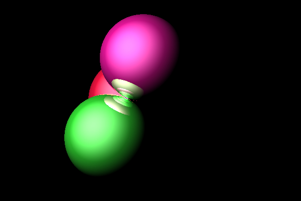
Which took 1m 3s to render.

Conclusion

So, what did we learn in this trip?

We can “parallelise” the constexpr evaluations by splitting the code into different static libraries. This ensures that the compiler uses multiple cores to generate the required libraries. As with most parallelisation, there is an ideal balance between the number of cores in the system and the number of libraries for optimum performance.

With this, we have concluded our journey. Could this be pushed further? Definitely! The current architecture actually gives us a lot more flexibility with the amount of features we can implement, since we no longer have to wait over 30 minutes per render. That said, we are still limited very limited in some ways. In particular:

Adding sampling increases the memory usage, which in turn limits the number of tiles we can have without the threads thrashing. This alone is the biggest limiting factor, since a low number of samples leads to a high amount of artefacts. The other consequence of this is that features such as ambient occlusion become either highly prohibitive or just impossible, since it relies very heavily on sampling. The same logic will apply with other sampling-heavy features.

So, if you’re interested, feel free to re-use the system we derived here for your own uses. If you do make something new, feel free to send me a link.

Well, that’s all for this series. Until we meet again, I bid you all a very fond farewell.

References

The following are the references used for this article in case you wish to read more about the discussed concepts.

Edits:
22/09/2024: Improved TOC and fixed some phrasing due to blog style changes.